Excel is a powerful tool for creating spreadsheets. How much of it do you use in your business?
Conditional formatting is one more technique you can use to add value to your spreadsheet and automate tasks. Lets say we have a spreadsheet where we want to track sales of a product over time. You want to highlight the days where you only sold ten items or less, to get an idea of which are good days and which are bad.
The slow solution is to go back after the data is entered and highlight the entries by formatting them with a green color if they are 10 or less.
Conditional formatting automates this task.
- Highlight the field or area you want to format.
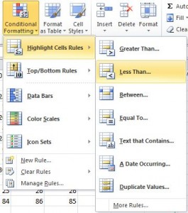
- Look for the Conditional Formatting button on your ribbon bar under Home.

Conditional Formatting Icon
- Select Highlight Cells Rule and then Less than…
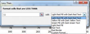
- For our example, I’ll type 11 in the box:

Entering the Condition
- Play around with the formatting options on the right or use a custom format.
Once finished, all the data in your highlighted area should be formatted based on your condition.
If you have any questions about any of our IT support tips, feel free to give me a call at (316) 337-5628 or our after hours support line at (316) 210-7112. We can walk you through this process, or talk to you about saving money on your IT support costs by moving to an affordable IT service provider in Wichita with no minimum service fees.

